1. Generative Modeling and Flow Matching
1.1. What is Generative Modeling?
Generative modeling is the process of learning how to sample data from the real-world data distribution. Technically speaking, it aims to transform samples from a simple, known distribution (e.g., standard Gaussian) into samples from a complex, unknown data distribution (e.g., CIFAR-10).
1.2. What We Have in Generative Modeling?
- An image dataset (empirical distribution of real-world data).
- A neural network (as a function approximator).
1.3. Why Using Flow Matching?
Traditional generative models like GANs and VAEs have their own strengths and limitations. Flow Matching offers a new perspective: instead of using adversarial training (like GAN) or encoders (like VAE), it directly learns a vector field guiding the points flow from noise to data.
This view naturally connects with differential equations and leads us to the core idea of flow matching: learning a neural ODE to model data generation. Flow Matching is also closely related to SDE-based diffusion models, as both methods involve transforming noise into data through continuous processes.
2. How Flow Matching Works for Generative Modeling?
Flow Matching learns a neural network to predict how a sample should move from noise point to data point, step by step, by simulating an ordinary differential equation (ODE).
2.1. ODE, Flow, and Vector Field
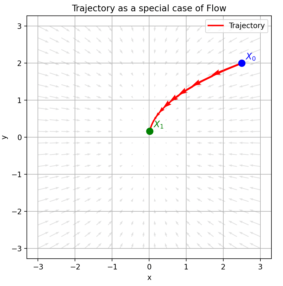
Figure 1. Illustration of vector field.
In order to understand flow matching thoroughly, let us start by understanding ordinary differential equations (ODEs). We can define a trajectory by a function $X: [0,1] \to \mathbb{R}^d (t \to X_t)$, which maps from time $t \in [0,1]$ to some location in $\mathbb{R}^d$. The trajectory is also a solution of the following ODE:
\[\frac{d X_t}{dt} = u_t(X_t), \quad s.t. \quad X_0 =x_0,\]where $X_0 =x_0$ means the starting point is $x_0$, $X_t$ tells us the position of a point at time $t$, given that it started at $x_0$. $u_t(X_t)$ is the velocity of the trajectory $X$ at time $t$.
For different starting point $x_0$, the trajectory $X_t$ will be different. We may ask that, for any starting point $x_0$, where is the position at time $t$? This requirs that $X_t$ is a function of time $t$ and the initial point $x_0$, we can rewrite it as $\psi_t(x_0)$, $\psi: [0,1]\times \mathbb{R}^d \to \mathbb{R}^d$, this function is also called flow, which is the solution of the following flow ODE:
\[\frac{d \psi_t(x_0)}{dt} = u_t(\psi_t(x_0)),\quad \psi_0(x_0) = x_0.\]$u_t(\cdot)$ defines a vector feild in $\mathbb{R}^d$ at time $t$ (at time $t$, for any point $\psi_t(x_0)\in \mathbb{R}^d$, $u_t(\psi_t(x_0))$ gives a velocity vector to tell the move direction).
In other word, vector fields defines ODEs whose solutions are flows!
2.2. Image Generation Process is a Flow
The process of transforming a noise sample $x_0$ into a data sample $x_1$ can be naturally interpreted as a flow – a continuous path governed by a vector field.
If we approximate the vector field $u_t(\cdot)$ with a neural network, for any strating point $x_0$, as $u_t(\cdot)$ tells us which direction we should move in, we can use numerical method such as Euler Method to simulate the ODE:
\[\psi_{t+h}(x_0) = \psi_{t}(x_0) +h \cdot u_t(\psi_t(x_0)), \quad (t=0,h,2h,\dots,1-h)\]$\psi_{0}(x_0)$ we already know is a noise, we can use the Euler Method to get $\psi_{1}(x_0)$ iteritively, that is the transformation of nosie into data.
In other words, if we know the direction in which each pixel should move at every moment during the continuous transformation from noise to data, we can transform any new noise sample into data sample. This is because we have learned the underlying ‘rule’ of the transformation — the velocity vector field.
2.3. Probability Path and Continuity Equation
Don’t forget our goal is transform samples from a known distribution (e.g., standard Gaussian) into samples from an unknown data distribution (e.g., CIFAR-10).
Now, let us consider a more complex scenario of flow: the starting points are sampled from a fixed distribution, e.g., $x_0 \sim \mathcal{N}(0,1)$, we konw every points will move in the space under the guidance of vetor field $u_t(\cdot)$, so the probability density of each point in the space will also change, thus, the data point distribution at each time $t$ is $p_t$ (i.e., $\psi_t(x_0) \sim p_t$), we call it probability path.
The probability density and the vector field satisfie the following key property (Continuity Equation):
\[\frac{\partial p_t(x)}{\partial t} =- \nabla_x \cdot (p_t(x)\cdot u_t(x))\]To provide an intuitive understanding of this equation, note that the left-hand side represents the instantaneous rate of change of the probability density at point $x$ over time. On the right-hand side, $p_t(x)$ denotes the probability density at position $x$, while $u_t(x)$ represents the velocity field–i.e., the speed and direction at which mass (or probability) moves at $x$. The product $p_t(x)\cdot u_t(x)$ describes the probability flux: it tells how much probability mass is flowing through space per unit time. Taking the divergence $\nabla \cdot (p_t(x) \cdot u_t(x))$ measures the net outflow of this flux from point $x$, and the negative sign indicates that when more mass flows out of $x$ than into it, the local density decreases accordingly.
That is to say, if we know $u_t$ and $p_0$, we can directly derive $p_t$; and if we just know $p_t$, we can solve the continuity equation to obtain a valid $u_t$ (the solution is not unique).
2.4. Conditional Probability Path and Conditional Vector Field
Now, let us consider to transform a sample from standard Gaussian distribution $p_0 = \mathcal{N}(0,1)$ into a sample from data distribution $p_1=p_{data}$, i.e., the probability path $p_t$ should satisfy: $p_0=p_{Gaussian}$, and $p_1=p_{data}$. If we can design a probability path $p_t$ with in a flow that satisfy the above two constraints (step 1), then we use a neural network to approximate the vector field $u_t(\cdot)$ (step 2), we will know how to generate data from noise!
- For step 1, unfortunately, we don’t know the analytic form of $p_{data}$, therefore we can’t create a parobability path $p_t$ directly (if we know, we can sample data from $p_{data}$ directly).
- For step 2, unfortunately, there is no analytic ground truth $u^{target}_t(\cdot)$ as supervision signal to train the neural network (if we know, why train a neural network to approximate it? just use it to generate data form noise using Euler Method mentioned in Section 3.2).
Fortunately, we have an image dataset, we can use it to learn $u^{target}_t(\cdot)$ implicitly.
2.4.1. Conditional Probability Path
Although we can’t design a probability path $p_t$, but we have an image dataset:
\[\mathcal{D} = \{z_1, z_2, \dots,z_n\}, \quad \forall i, z_i \sim p_{data}\]for a give data $z$, we can define the conditional probability path $p_t(\cdot \mid z)$, and we know:
\[p_t(\cdot) = \mathbb{E}_{z\sim p_{data}}[p_t(\cdot \mid z)] = \int p_t(x \mid z) \cdot p_{data}(z) dz\]If we set $p_0(\cdot \mid z) = \mathcal{N}(0, 1)$, then
\[p_0(\cdot) = \mathbb{E}_{z\sim p_{data}}[p_0(\cdot \mid z)] = p_0(\cdot \mid z)=\mathcal{N}(0, 1)\]is also a standard Gaussian distribution.
Similarly, we can set $p_1(\cdot \mid z) = \delta_z$ (Dirac delta distribution, sampling from $\delta_z$ always returns $z$), then
\[p_1(\cdot) = \mathbb{E}_{z\sim p_{data}}[p_1(\cdot \mid z)] = p_{data}(z)=p_{data}\]Such a conditional probability path $p_t(\cdot \mid z)$ is easy to design, for example, we can use a linear interpolation between $\mathcal{N}(0,1)$ and $\delta(z)$:
\[p_t(x \mid z) = (1-t) \cdot \mathcal{N}(0, 1) + t \cdot \delta_z(x) = \mathcal{N}(t\cdot z, (1-t)^2 I_d), \quad t\in[0,1].\]As you can see, if we design such a conditional probability path $p_t(\cdot \mid z)$, the marginal probability path $p_t(\cdot)$ will satisfy the constraints we need. And we can sample from $p_t(\cdot)$ by first sampling a data point $z$ from $p_{data}$, and then sample a point $x$ from $p_t(\cdot \mid z)$. We have designed an conditional probability path $p_t(\cdot \mid z)$, which induces a valid probability path $p_t(\cdot)$ we need. However, we can’t access the analytic form of $p_t(\cdot)$ as the integral is intractable.
2.4.2. Conditional Vector Field
Now, let us construct a valid conditional vector field for the designed conditional probability path. The corresponding conditional vector field can, in principle, be obtained by solving the continuity equation. However, in this example, we can easily observe that our conditional probability path can be induced by the following simple conditional flow directly (the valid conditional flow is not unique):
\[\psi_t(x_0 \mid z) = (1-t) \cdot x_0 + t\cdot z.\]if $X_0 \sim \mathcal{N}(0,1)$, then $X_t \sim \mathcal{N}(t\cdot z, (1-t)^2 I_d)=p_t(\cdot \mid z)$.
Therefore, by definition, we can extract the target conditional vector field:
\[\frac{d}{d t} \psi_t(x_0 \mid z) = u_t(\psi_t(x_0 \mid z) \mid z), \forall x, z \in \mathbb{R}^d\]let $x_t = \psi_t(x_0 \mid z) = (1-t) \cdot x_0 + t\cdot z$, we have:
\[\begin{aligned} \frac{d}{d t} \psi_t(x_0 \mid z) = u_t(x_t \mid z) &= \frac{d}{d t} \left ((1-t) \cdot x_0 + t\cdot z \right ) \\ & = z - x_0. \end{aligned}\]That is to say:
\[\begin{aligned} u_t(x_t \mid z) &= z-x_0, \quad s.t. \quad x_t = (1-t) \cdot x_0 + t \cdot z \end{aligned}\]is a valid conditional vector field, it defines an ODE which solution is the conditional flow: $\psi_t(x_0 \mid z) = (1-t) \cdot x_0 + t\cdot z$, and the flow induced a conditional probability path: $p_t(\cdot \mid z) = \mathcal{N}(t\cdot z, (1-t)^2 I_d)$.
2.5. Approximation of Vector Field
As described in section 2.2, we want to train a neural network $u^{\theta}_t(x_t)$ to approximate the vector field $u^{target}_t(x_t)$, we can achieve this by optimizing the following loss function:
\[\begin{aligned} \mathcal{L}_{FM} (\theta) &= \mathbb{E}_{t\sim U[0,1], x_t \sim p_t} \left \| u^{\theta}_t(x_t) - u^{target}_t(x_t) \right \|^2 \\ &= \mathbb{E}_{t\sim U[0,1], z \sim p_{data}, x_t \sim p_t(\cdot \mid z)} \left \| u^{\theta}_t(x_t) - u^{target}_t(x_t) \right \|^2. \end{aligned}\]Unfortunately, As discussed earlier, the ground truth $u^{target}_t(x_t)$ is unknown, we only have an conditional ground truth vector field: $u_t(x_t \mid z) = z-x_0 \quad (s.t. \quad x_t = (1-t) \cdot x_0 + t \cdot z)$, a natural question is: what will happen if we optimize the following loss function:
\[\begin{aligned} \mathcal{L}_{CFM} (\theta) &= \mathbb{E}_{t\sim U[0,1], z \sim p_{data}, x_t \sim p_t(\cdot \mid z)} \left \| u^{\theta}_t(x_t) - u^{target}_t(x_t \mid z) \right \|^2 \\ &= \mathbb{E}_{t\sim U[0,1], z \sim p_{data}, x_t \sim p_t(\cdot \mid z)} \left \| u^{\theta}_t(x_t) - (z - x_0) \right \|^2. \end{aligned}\]The answer is: optimizing \(\mathcal{L}_{FM} (\theta)\) is equivalent to optimizing \(\mathcal{L}_{CFM} (\theta)\).
Let us give a formal proof of the above result.
To prove the equivalence of FM and CFM loss, we apply the marginalization trick and rewrite expectations. The key idea is to decompose the marginal loss via the law of total expectation.
First, let us introduce a key lemma, which reveals the relationship of conditional vector field $u_t(x \mid z)$ and (marginal) vector field $u_t(x)$:
Lemma 1. (marginalization trick). For every data point $z \in \mathbb{R}^d$, let $u^{target}_{t}(\cdot \mid z)$ denote a conditional vector field, defined so that the corresponding ODE yields the conditional probability path $p_t(\cdot \mid z)$, we have:
\[u^{target}_t(x) = \int u^{target}_{t}(x \mid z) \cdot \frac{p_t(x \mid z)\cdot p_{data}(z)}{p_t(x)}dz.\]Proof.
\[\begin{aligned} \frac{\partial p_t(x)}{\partial t} &= \frac{\partial \int_z p_t(x \mid z)p_{data}(z)dz}{\partial t} && \text{(by definition)}\\ &= \int_z \frac{\partial p_t(x \mid z)}{\partial t} p_{data}(z) dz && \text{(swap the order of integral and differential)}\\ &= \int_z (- \nabla_x \cdot (p_t(x \mid z)\cdot u_t(x \mid z))) p_{data}(z)dz && \text{(continuity equation)}\\ &= - \nabla_x \cdot \int_z (p_t(x \mid z)\cdot u_t(x \mid z)) p_{data}(z)dz && \text{(swap the order of integral and differential)}\\ &= - \nabla_x \cdot \left( p_t(x) \int_z u_t(x \mid z) \cdot \frac{p_t(x \mid z) \cdot p_{data}(z)}{p_t(x)}dz \right),\\ \end{aligned}\]as we kown (continuity equation): $\frac{\partial p_t(x)}{\partial t} = - \nabla_x \cdot (p_t(x) \cdot u_t(x))$, therefore:
\[\begin{aligned} - \nabla_x \cdot \left( p_t(x) \int u_t(x \mid z) \cdot \frac{p_t(x \mid z) \cdot p_{data}(z)}{p_t(x)}dz \right) &= - \nabla_x \cdot (p_t(x) \cdot u_t(x)) \\ \Rightarrow \int u_t(x \mid z) \cdot \frac{p_t(x \mid z) \cdot p_{data}(z)}{p_t(x)}dz &= u_t(x). \end{aligned}\]Q.E.D.
Now, we prove the following main theorem:
Theorem 1. The marginal flow matching loss equals the conditional flow matching loss up to a constant:
\[\mathcal{L}_{FM} (\theta) = \mathcal{L}_{CFM} (\theta) + C\]Proof.
\[\begin{aligned} \mathcal{L}_{FM} (\theta) &= \mathbb{E}_{t\sim U[0,1], x \sim p_t} \left \| u^{\theta}_t(x) - u^{target}_t(x) \right \|^2 \\ (\text{Sampling trick})&= \mathbb{E}_{t\sim U[0,1], z \sim p_{data}, x \sim p_t(\cdot \mid z)} \left \| u^{\theta}_t(x) - u^{target}_t(x) \right \|^2\\ (\left \| a - b\right \|^2 = a^2 - 2 a^T b + b^2)&= \mathbb{E}_{t\sim U[0,1], z \sim p_{data}, x \sim p_t(\cdot \mid z)} \left [ \left \| u^{\theta}_t(x)\right \|^2 - 2\cdot u^{\theta}_t(x)^{T}\cdot u^{target}_t(x) + \underbrace{\left \| u^{target}_t(x)\right \|^2}_{\theta \text{-independent constant}} \right ] \\ &= \mathbb{E}_{t\sim U[0,1], z \sim p_{data}, x \sim p_t(\cdot \mid z)} \left [ \left \| u^{\theta}_t(x)\right \|^2 - 2\cdot u^{\theta}_t(x)^{T}\cdot u^{target}_t(x) \right ] + C_1 \\ (\text{Expectation definition})& = \mathbb{E}_{t\sim U[0,1], z \sim p_{data}, x \sim p_t(\cdot \mid z)} \left \| u^{\theta}_t(x)\right \|^2 - \int^{1}_{0} \int \int \left ( 2\cdot u^{\theta}_t(x)^{T}\cdot u^{target}_t(x) \right ) \cdot p_t(x \mid z) \cdot p_{data}(z) dz dx dt + C_1\\ (\text{Lemma 1})&=\mathbb{E}_{t\sim U[0,1], z \sim p_{data}, x \sim p_t(\cdot \mid z)} \left \| u^{\theta}_t(x)\right \|^2 - \int^{1}_{0} \int \int 2\cdot u^{\theta}_t(x)^{T}\cdot \int u_t^{target}(x \mid z) \cdot \frac{p_t(x \mid z) \cdot p_{data}(z)}{p_t(x)}dz \cdot p_t(x \mid z) \cdot p_{data}(z) dz dx dt + C_1\\ &=\mathbb{E}_{t\sim U[0,1], z \sim p_{data}, x \sim p_t(\cdot \mid z)} \left \| u^{\theta}_t(x)\right \|^2 - \int^{1}_{0} \int \int 2\cdot u^{\theta}_t(x)^{T}\cdot u_t^{target}(x \mid z) \cdot p_t(x \mid z) \cdot p_{data}(z) dz dx dt + C_1\\ &=\mathbb{E}_{t\sim U[0,1], z \sim p_{data}, x \sim p_t(\cdot \mid z)} \left \| u^{\theta}_t(x)\right \|^2 - \mathbb{E}_{t\sim U[0,1], z \sim p_{data}, x \sim p_t(\cdot \mid z)} \left [2\cdot u^{\theta}_t(x)^{T}\cdot u_t^{target}(x \mid z) \right ] + C_1\\ &= \mathbb{E}_{t\sim U[0,1], z \sim p_{data}, x \sim p_t(\cdot \mid z)} \left [ \left \| u^{\theta}_t(x)\right \|^2 - 2\cdot u^{\theta}_t(x)^{T}\cdot u_t^{target}(x \mid z) + \left \|u_t^{target}(x \mid z)\right \|^2 - \left \|u_t^{target}(x \mid z)\right \|^2 \right] + C_1\\ &= \mathbb{E}_{t\sim U[0,1], z \sim p_{data}, x \sim p_t(\cdot \mid z)} \left [ \left \| u^{\theta}_t(x) - u_t^{target}(x \mid z)\right \|^2 \right] - \underbrace{\mathbb{E}_{t\sim U[0,1], z \sim p_{data}, x \sim p_t(\cdot \mid z)} \left \|u_t^{target}(x \mid z)\right \|^2}_{\theta \text{-independent constant}} + C_1\\ &= \mathbb{E}_{t\sim U[0,1], z \sim p_{data}, x \sim p_t(\cdot \mid z)} \left [ \left \| u^{\theta}_t(x) - u_t^{target}(x \mid z)\right \|^2 \right] + C\\ &= \mathcal{L}_{CFM}(\theta) + C \end{aligned}\]Q.E.D.
3. Summary and Further Readings
We introduced the principle of Flow Matching from the ground up: from vector fields and flows to the design of conditional paths and training loss. By understanding its mathematical foundation, we can better appreciate its connection to score-based models, diffusion, and neural ODEs.
If you’re interested in further exploring Flow Matching, you may want to check: