Overview
In this post, we will explore the concept of PAC (Probably Approximately Correct) learnability, specifically focusing on the learnability of axis-aligned rectangles in a two-dimensional space. We will provide a simplified definition of PAC learnability, describe the rectangle concept class, and prove that it is PAC-learnable using a specific learning algorithm. This proof will illustrate key techniques commonly used in PAC learning proofs.
1. Simplified Definition of PAC Learnability (Sample Complexity Only)
1.1. Generalization Error
Definition 1. (Generalization Error) Given a hypothesis $h \in \mathcal{H}$, a target concept $c \in \mathcal{C}$, and an underlying distribution $\mathcal{D}$ over the input space $\mathcal{X}$, the generalization error (or risk) of $h$ with respect to $c$ is defined as:
\[Risk(h) = \mathbb{P}_{x \sim \mathcal{D}} [h(x) \neq c(x)] = \mathbb{E}_{x \sim \mathcal{D}} [\mathbb{I}(h(x) \neq c(x))]\]1.2. PAC Learnability
Definition 2. (PAC Learnability) A concept class $\mathcal{C}$ is said to be PAC-learnable if there exists a learning algorithm $\mathcal{A}$ and a polynomial function $poly(\cdot,\cdot)$, such that for all distributions $\mathcal{D}$ over the input space $\mathcal{X}$, for any concept $c \in \mathcal{C}$, for any $\epsilon, \delta > 0$, the following holds for any sample size $m \geq poly(\frac{1}{\epsilon}, \frac{1}{\delta})$:
\[\Pr_{S \sim \mathcal{D}^m} [Risk(h_S) \leq \epsilon] \geq 1 - \delta\]where $h_S$ is the hypothesis learned from sample $S$ through $\mathcal{A}$, and $Risk(h_S)$ is the risk of the hypothesis.
To put it simply, a concept class is PAC-learnable if there exists a learning algorithm that can approximate any concept in the class within a small error margin with high probability, given a sufficiently large sample size (but not exceeding the polynomial bounds).
2. The Rectangle Concept Class Case
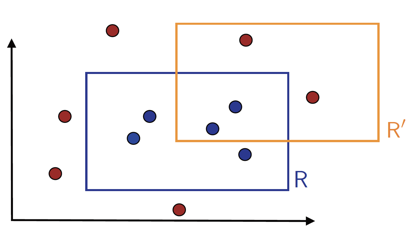
Figure 1. Target concept R and the learned hypothesis R'.
Example (Learning axisaligned rectangles) As shown in Figure 1, consider the case where the set of instances are points in the $\mathbb{R}^2$ space, and the concept class $\mathcal{C}$ is the set of all axis-aligned rectangles lying in $\mathbb{R}^2$. Thus, each concept $c$ is the set of points inside a particular axis-aligned rectangle. The learning problem consists of determining with small error a target axis-aligned rectangle using the labeled training sample. Note that, we assume there exists a target rectangle $c^*$ that can discriminate the positive and negative examples perfectly.
We will show that the concept class of axis-aligned rectangles is PAC-learnable.
2.1. Learning Algorithm
First, we define the learning algorithm $\mathcal{A}$, which takes as input a labeled sample $\mathcal{S} \sim \mathcal{D}^m$ and outputs a hypothesis $h$ corresponding to the tightest axis-aligned rectangle enclosing the positive examples.
\[\begin{array}{l} \textbf{Algorithm 1: Find the Consistent Rectangle} \\ \textbf{Input:} \text{Sample } S = \{(x_1, y_1), \ldots, (x_n, y_n)\}, x_i \in \mathbb{R}^2, y_i \in \{0,1\} \\ \textbf{Output:} \text{Axis-aligned rectangle } R \\[1ex] 1.\quad R \gets \text{Smallest axis-aligned rectangle enclosing all } x_i \text{ such that } y_i = 1 \\ 2.\quad \textbf{return } R \end{array}\]2.2. Proving PAC Learnability
Now, we will prove that this algorithm PAC-learns the axis-aligned rectangle concept class.
Let $R \in \mathcal{C}$ be a target concept, and let $R’$ be the learned hypothesis from the sample $\mathcal{S}$ using Algorithm 1.
By definition, we know the following statement is true:
- $R’$ will not produce any false negatives (on $\mathcal{S}$), i.e., it will include all points that are labeled as positive in the sample. So, $R’$ will be included in the target rectangle $R$, as shown in Figure 2. This implies that errors can only arise in the region that lies inside the target concept rectangle but outside the hypothesis rectangle.
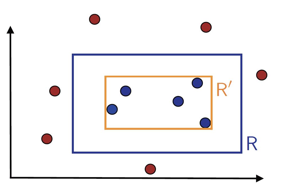
Figure 2. Illustration of the hypothesis R' returned by algorithm 1.
For any fixed $\epsilon > 0$, we want to know the probability of generalization error $Risk(R’) \le \epsilon$. If the probability of the target rectangle $\mathbb{P}[R] \le \epsilon$, then the generalization error $Risk(R’)$ will never exceed $\epsilon$, which means $\mathbb{P}[Risk(R’) \le \epsilon] = 1$, it is trivially true. So, we need assume that the target rectangle $R$ is not too small, i.e., $\mathbb{P}[R] > \epsilon$. Now, since $\mathbb{P}[R] > \epsilon$, we proceed to bound the probability of the generalization error $Risk(R’)$.
As shown in Figure 3, we define four rectangular regions $r_1$, $r_2$, $r_3$, and $r_4$ along each side of the target rectangle $R$, as shown in Figure 3. Moreover, we ensure each of these regions with probability at least $\frac{\epsilon}{4}$, i.e., $\forall i \in [4], \mathbb{P}[r_i] \ge \frac{\epsilon}{4}$. Meanwhile, $\mathbb{P} [\bigcup_{i=1}^{4} r_i] < \epsilon$. It is worth noting that these regions can indeed be constructed, as $\mathbb{P}[R] > \epsilon$. (one region can be constructed by starting with the full rectangle $R$ and then decreasing the size by moving one side as much as possible while keeping the probability at least $\frac{\epsilon}{4}$).
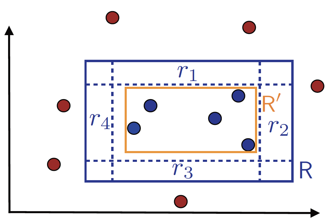
Figure 3. Illustration of the constructed regions r_i.
Now, we know that the proposition $P \to Q$ is true, where
- Event $P$: Each of the four regions $r_i$ contains at least one sample in $\mathcal{S}$.
- Event $Q$: The generalization error $Risk(R’) \le \epsilon$.
as $\mathbb{P} [\bigcup_{i=1}^{4} r_i] < \epsilon$, if $P$ is true, the error region of the hypothesis $R’$ will be a subset of the union of $\bigcup_{i=1}^{4} r_i$. Thus, the probability of the error region will be less than $\epsilon$, i.e., $Risk(R’) < \epsilon$, which means $Q$ is true. Additionally, we define event $\bar P$: There exists at least one region among $r_1, r_2, r_3, r_4$ that contains no sample, which denotes the complement of event $P$. Let event $A_i$ be the event that the region $r_i$ contains no sample, and $\delta > 0$. Then, We have:
\[\begin{aligned} \mathbb{P}[Risk(R') \le \epsilon] &= \mathbb{P}[Q] && \text{(by definition of Q)} \\ &\overset{(i)}{\ge} \mathbb{P}[P] \\ &\overset{(ii)}{=} 1 - \mathbb{P}[\bar P] \\ &\overset{(iii)}{=} 1 - \mathbb{P}\left [\bigcup_{i=1}^{4} A_i \right ] \\ &\overset{(iv)}{\ge} 1 - \sum_{i=1}^{4} \mathbb{P}\left [A_i \right ] \\ &\overset{(v)}{=} 1 - 4 (1 - \frac{\epsilon}{4})^m \\ &\overset{(vi)}{\ge} 1 - 4 exp(\frac{-m\cdot \epsilon}{4}) \\ \end{aligned}\]where in (i) we use the fact that $P \subseteq Q$, in (ii) we use the fact that $\mathbb{P}[P] = 1 - \mathbb{P}[\bar P]$, in (iii) we rewrite the term, in (iv) we use the the union bound, in (v) we use the fact that $\mathbb{P}[A_i] = (1 - \frac{\epsilon}{4})^m$, and in (vi) we use the fact that $1 - x \le exp(-x)$ for any $x > 0$.
If we impose that $\mathbb{P}[Risk(R’) \le \epsilon] = 1 - 4 exp(\frac{-m\cdot \epsilon}{4}) \ge 1 - \delta$, which will be satisfied if:
\[4 exp(\frac{-m\cdot \epsilon}{4}) \le \delta \\ \Leftrightarrow m \ge \frac{4}{\epsilon} \log(\frac{4}{\delta})\]Therefore, we can conclude that the concept class of axis-aligned rectangles is PAC-learnable with the sample complexity of $m \ge \frac{4}{\epsilon} \log(\frac{4}{\delta})$.
Q.E.D.
2.3. Tricks for PAC Learning Proofs
- (1) Introduce the concept of “error region” is a common technique in PAC learning proofs.
- (2) The union bound is a powerful tool to bound the probability of the union of events.
- (3) Keep in mind the relationship between the probability of an event and its complement, i.e., $\mathbb{P}[A] = 1 - \mathbb{P}[\bar A]$, which is often used to construct “$1 - X$” form, such as step (ii) and (v) in our proof.
- (4) The exponential bound $1 - x \leq exp(-x)$ is often used in the last step to simplify the expression and obtain a bound on the probability.
3. Aknowledgements
This post is written with reference to: